
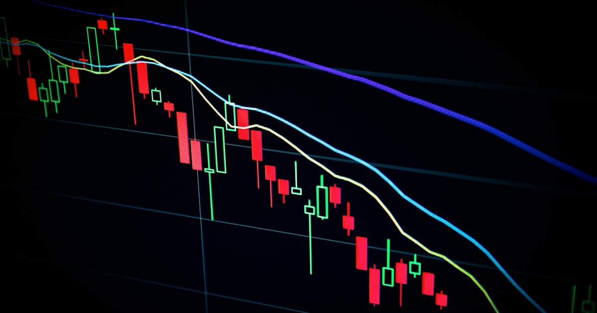
TL;DR. Bollinger Bands wrap a moving average of price in two lines drawn at plus and minus a chosen number of standard deviations. The default set-up — a 20-period simple moving average with bands at ±2 standard deviations — is the same one John Bollinger published more than three decades ago and remains unchanged today. The bands are not buy or sell signals. They are a relative definition of high and low that traders combine with other tools to spot pattern setups such as the “squeeze,” walking the bands in a trend, and M-tops and W-bottoms. Retail traders most often go wrong by treating band touches as automatic reversals and by assuming the ±2σ math implies a 95% containment probability. It doesn’t.
What Bollinger Bands actually measure
Bollinger Bands were introduced by John Bollinger in the early 1980s and have since become one of the most widely charted technical indicators on Wall Street. The construction is deliberately simple: a moving average of price runs down the middle, and two envelopes above and below it move in and out as recent price volatility rises and falls. When price is placid, the bands narrow. When price is jumpy, the bands widen. The width of the envelope is the volatility read.
Bollinger himself is emphatic about what the bands are for. In Rule 1 of his 22 rules for using the bands, he writes that the bands “provide a relative definition of high and low. By definition, price is high at the upper band and low at the lower band.” That is a comparative statement about where price sits right now relative to its own recent range — not a forecast (bollingerbands.com — 22 rules).
The SEC’s investor-education arm reminds retail investors that technical indicators analyse past price patterns and are not, on their own, forecasts of future returns (SEC Investor.gov).
The formula, line by line
All three lines are computed from the same input — the closing price — on a rolling window of N periods:
- Middle band = N-period simple moving average (SMA) of close.
- Upper band = middle band + k × standard deviation of close over the same N periods.
- Lower band = middle band − k × standard deviation of close over the same N periods.
Bollinger’s default is N = 20 and k = 2. He notes on his own site that these defaults “today are the same as they were 35 years ago” (bollingerbands.com).
The standard deviation is computed on the same 20 closes used for the SMA — it is the population standard deviation of that rolling window, not a look-ahead estimate. Because the deviation is recomputed every bar, the bands expand and contract in real time as the market’s recent volatility changes.
A worked example
Suppose the last 20 daily closes of a stock have a mean of $100.00 and a standard deviation of $2.00. Then, on that bar:
- Middle band = $100.00
- Upper band = 100.00 + 2 × 2.00 = $104.00
- Lower band = 100.00 − 2 × 2.00 = $96.00
If, over the next several sessions, price becomes calmer and the rolling standard deviation falls from $2.00 to $0.75 while the mean stays near $100, the bands compress to roughly $101.50 / $98.50 — a much tighter envelope. This narrowing is what Bollinger calls the squeeze, and it is his indicator’s most-referenced setup (see chart below).
Two derived indicators worth knowing
Bollinger himself popularised two derived series that sit alongside the bands on many charting packages:
- %b normalises where price sits inside the envelope: %b = (Close − Lower) / (Upper − Lower). A %b of 1.0 means price is exactly at the upper band; 0.0 means it is at the lower band; values below 0 or above 1 mean price has closed outside the bands.
- BandWidth measures the width of the envelope, normalised by the middle band: BandWidth = (Upper − Lower) / Middle. Bollinger notes that BandWidth’s “most popular use is to identify ‘The Squeeze’” — the compression that often precedes a large move (bollingerbands.com — Rule 18).
Parameter presets in the wild
Bollinger explicitly cautions against changing parameters casually. Rule 9 states that the default 20/2 “are just that, defaults” — adjustable, but with care. Rule 11 adds that if you change the length of the middle band, you should also adjust the standard-deviation multiplier so the envelope still captures a comparable share of price action. The table below shows the default alongside two variants that appear frequently in charting-package presets.
| Preset | Period (N) | Std-dev multiplier (k) | Typical use |
|---|---|---|---|
| Bollinger default | 20 | 2.0 | Daily charts; general use |
| Shorter-term variant | 10 | 1.9 | Intraday and swing setups |
| Longer-term variant | 50 | 2.1 | Position trading; weekly context |
How the bands look on a chart
The clearest way to see what the envelope is doing is to draw it. In the SVG below, a stylised price series (the dark line) walks inside a 20-period Bollinger envelope. Notice the shape of the setup: price rides the upper band during a trend, pulls back to the middle band, then compresses inside a tight envelope before a fresh expansion. That compression is the squeeze.
The three canonical setups
1. Walking the bands
In a strong trend, price can hug — and repeatedly close above — the upper band for many sessions in a row (or the lower band in a downtrend). Bollinger’s Rule 7 makes this explicit: “In trends, price can, and does, walk up the upper Bollinger Band and walk down the lower Bollinger Band.” Rule 8 adds that closes outside the bands are continuation signals, not reversal signals. Selling every tag of the upper band in a strong uptrend is a classic way to give money away.
2. The squeeze
When BandWidth compresses to a multi-month low, historical volatility has fallen and the market is coiled. A break of the compressed range — either above the upper band or below the lower band — often marks the start of a new directional move. The squeeze is not, by itself, a trade: Bollinger stresses that direction must be confirmed by other tools (volume, momentum oscillators, price structure).
3. M-tops and W-bottoms
Rule 5 says: “Bollinger Bands can be used to clarify pure price patterns such as M-type tops and W-type bottoms.” In a classic W-bottom, price makes a low that pierces the lower band, rallies, then re-tests the low — but the second low does not pierce the band. The pattern gains conviction when %b makes a higher low even as price makes a lower low: momentum has diverged from price, and the second low sits deeper inside the envelope than the first. M-tops mirror the setup on the upside.
The mistakes retail traders make with Bollinger Bands
Treating band touches as buy or sell signals
This is the single most common misuse. Rule 6 could not be plainer: “Tags of the bands are just that, tags, not signals.” A tag of the upper band during a strong trend often marks the start of the move, not the end of it. In a genuine range-bound market, tags do have more predictive value — but the trade still needs confirmation from a second, unrelated indicator, such as an oscillator or a volume series (Rule 3).
Assuming ±2σ contains 95% of price
For a normal distribution, roughly 95.45% of observations sit within two standard deviations of the mean (Wikipedia: 68–95–99.7 rule). Stock prices are famously not normal — returns have fat tails, and the mean itself is moving. In practice, the share of bars that close inside a 20/2 Bollinger envelope is materially less than 95%. Bollinger’s own Rule 14 says it directly: “Do not make statistical assumptions based on the use of the standard deviation calculation in the construction of the bands.” The bands are a relative range measure, not a probabilistic confidence interval.
Using it in isolation
Bollinger’s Rule 3 recommends deriving confirmation indicators from a different input category — momentum, volume, sentiment, or open interest — rather than layering multiple price-derived tools that all say the same thing. Two moving averages plus MACD plus Bollinger Bands is not four opinions; it is one opinion counted four times.
Over-optimising the parameters
Traders who back-test dozens of period/multiplier combinations on the same instrument almost always find a “best” setting that fits the last few years of data and fails out of sample. Bollinger’s own defaults have survived four decades of markets because they were chosen for robustness, not curve-fit performance.
What to pair Bollinger Bands with
Because the bands describe where price is inside its own recent volatility, the natural pairings are indicators that describe why or with what conviction price is moving there:
- Volume — a squeeze breakout on rising volume is a stronger setup than the same breakout on falling volume.
- Momentum oscillators (RSI, MACD) — useful for confirming M-tops and W-bottoms via divergence, per Bollinger’s Rule 5.
- Price structure — horizontal support and resistance, prior swing highs, and volume-profile levels turn a “band tag” into a defined trade with a stop and a target.
Related concepts and what to learn next
- MACD, another Appel-era indicator that pairs cleanly with Bollinger Bands. See our companion piece: MACD Explained: Formula, Signals, and Common Pitfalls.
- The VIX and implied volatility, which describe forward-looking volatility rather than the trailing realised volatility that Bollinger Bands measure. See: The VIX Explained: How Wall Street’s Fear Gauge Works.
- Standard deviation, the primary building block, and why financial return distributions violate the tidy assumptions taught in most statistics classes.
Sources
- John Bollinger — The default parameters of Bollinger Bands. bollingerbands.com. Confirms 20-period simple moving average and ±2 standard-deviation defaults, unchanged for more than 30 years.
- John Bollinger — 22 rules for using Bollinger Bands. bollingerbands.com. Source for Rules 1, 3, 5, 6, 7, 8, 9, 11, 14, and 18 referenced above.
- Wikipedia — 68–95–99.7 rule. Source for the normal-distribution ±2σ ≈ 95.45% statistic.
- U.S. Securities and Exchange Commission — Investor.gov glossary: technical analysis. Investor-education context on the role of technical indicators.
Disclosure: This article is for informational purposes only and is not investment advice.