Category: Market Education

  • Investor Psychology: Navigating Fear, Greed, and Market Sentiment Cycles

    Investor Psychology: Navigating Fear, Greed, and Market Sentiment Cycles

    Mastering Emotional Intelligence in Financial Markets

    Financial success isn’t just about analyzing balance sheets, tracking market trends, or understanding economic indicators—it’s fundamentally about mastering your own psychology. While textbooks and finance courses teach valuation models and technical analysis, they rarely address the powerful emotional forces that drive the majority of investment decisions. Fear, greed, overconfidence, and herd mentality repeatedly cause rational investors to make irrational choices, turning promising investment strategies into disappointing losses. Understanding investor psychology—the behavioral patterns, cognitive biases, and emotional cycles that govern market participants—is perhaps the most valuable yet underappreciated skill in successful investing. Whether you’re navigating a market panic, resisting FOMO during a speculative bubble, or fighting the urge to sell during temporary downturns, your ability to recognize and manage psychological forces determines your long-term investment success.

    The Psychology of Investing

    Investor psychology examines how human emotions, cognitive biases, and behavioral patterns influence financial decision-making. Unlike traditional finance theory, which assumes investors are rational actors who consistently make optimal choices, behavioral finance recognizes that humans are deeply emotional, frequently irrational, and systematically prone to predictable mistakes.

    These psychological factors manifest in several powerful ways:

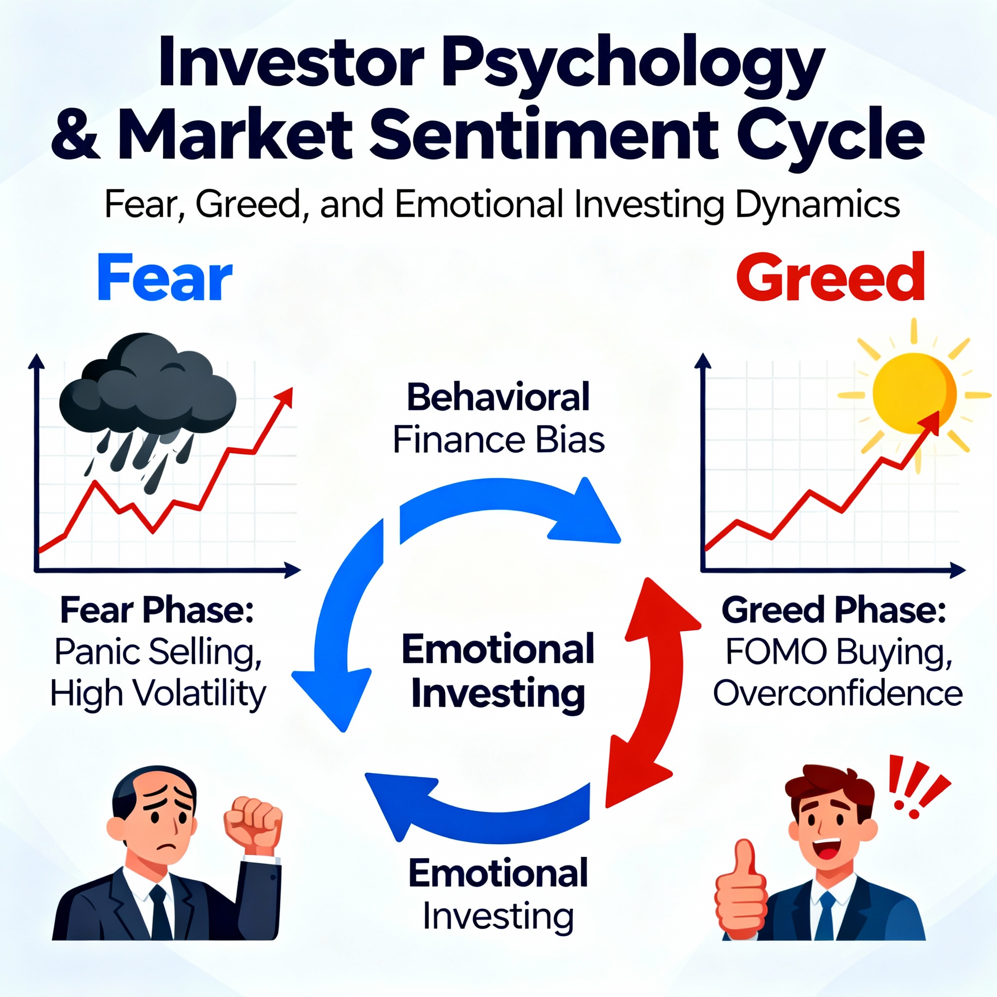
    Emotional Decision-Making: Fear and greed overwhelm rational analysis during market extremes. When markets crash, fear triggers panic selling at precisely the wrong time. When markets soar, greed fuels speculative buying at peak valuations.

    Cognitive Biases: Mental shortcuts and systematic thinking errors lead investors astray. Confirmation bias causes investors to seek information supporting existing beliefs while ignoring contradictory evidence. Recency bias makes recent market performance feel more important than long-term historical patterns.

    Herd Behavior: Social pressure and fear of missing out drive investors to follow the crowd rather than conducting independent analysis. This collective behavior creates bubbles during euphoric periods and crashes during panic phases.

    Market Sentiment Cycles

    Markets don’t move in straight lines—they oscillate through predictable psychological cycles as investor sentiment swings between extreme optimism and extreme pessimism. Understanding these sentiment cycles helps investors recognize where markets stand emotionally and position themselves accordingly.

    The typical market sentiment cycle progresses through distinct phases:

    Optimism: Markets begin recovering from previous lows. Early investors recognize value and accumulate positions. Sentiment improves gradually as prices rise and fear subsides.

    Excitement: Prices accelerate higher. Media coverage turns increasingly positive. More investors join the rally, pushing prices further upward. Skepticism diminishes as gains continue.

    Thrill: Markets surge dramatically. Everyone seems to be making money. Investor confidence reaches extreme levels. Risk-taking behavior intensifies as fear disappears almost entirely.

    Euphoria: Peak sentiment—maximum financial risk coincides with maximum psychological comfort. Investors believe “this time is different” and markets can only go higher. Speculative excess reaches extreme levels. THIS is when smart money begins exiting.

    Anxiety: First cracks appear. Prices begin falling from highs. Investors initially dismiss declines as “healthy corrections” or “buying opportunities,” but doubt creeps in as losses mount.

    Denial: Losses deepen but investors refuse to accept changing conditions. “The market will bounce back” becomes the common refrain. Many hold losing positions, hoping for recovery rather than accepting reality.

    Fear: Panic sets in as losses accelerate. Investors desperately seek ways to protect remaining capital. Selling pressure intensifies, creating downward spirals.

    Desperation: Markets reach deeply oversold levels. Investors feel helpless as portfolios decline relentlessly. Capitulation—the final surrender where remaining holders throw in the towel—approaches.

    Panic/Capitulation: Maximum fear coincides with maximum opportunity. Everyone wants out. Prices reach irrational lows as indiscriminate selling dominates. THIS is when smart money accumulates.

    Despondency: After the crash, investors remain traumatized. Even as values recover, fear keeps many sidelined. Market participation drops to low levels.

    Depression: Pessimism dominates. Investors swear off stocks entirely. Media declares “the end of the bull market era.” THIS pessimism creates the foundation for the next cycle.

    Hope: Green shoots emerge. A few brave investors begin accumulating quality assets at depressed valuations. The cycle begins anew.

    Herd Behavior and FOMO

    Herd behavior—the tendency to follow the crowd rather than making independent decisions—represents one of investing’s most dangerous psychological traps. This behavior stems from deep evolutionary instincts: for most of human history, following the group enhanced survival. But in financial markets, following the herd systematically destroys wealth.

    Herd behavior manifests most dramatically during market extremes:

    Bubbles: Everyone rushes into the “hot” asset class simultaneously. Dot-com stocks in 1999, real estate in 2006, cryptocurrencies in 2021—each bubble featured investors abandoning fundamental analysis and piling into overvalued assets simply because “everyone else is doing it.”

    Crashes: Panic becomes contagious. When prices fall, mass selling creates self-reinforcing downward spirals. The 2020 COVID crash saw even long-term investors dump quality stocks at fire-sale prices out of pure fear.

    FOMO (Fear of Missing Out) amplifies herd behavior during euphoric phases. As investors watch others apparently getting rich, psychological pressure to join intensifies:

    “My neighbor made a fortune in Bitcoin—I should buy some too!”
    “GameStop is up 400%—I’m missing out!”
    “Everyone’s talking about this hot IPO—I need to get in!”

    FOMO-driven decisions typically occur at precisely the worst times—near market tops when risk is highest and expected returns are lowest. The antidote to FOMO is understanding that missing a speculative rally is vastly preferable to participating in the inevitable crash that follows.

    Key Formulas and Concepts

    While psychology resists mathematical formulas, behavioral finance has identified quantifiable patterns in irrational behavior:

    Loss Aversion

    Psychological research demonstrates that losses hurt approximately twice as much as equivalent gains feel good. This asymmetry explains why investors hold losing positions too long (refusing to accept painful losses) while selling winners too quickly (eager to lock in pleasurable gains).

    Loss Aversion Ratio ≈ 2:1

    Pain from $1,000 loss > Pleasure from $1,000 gain

    This mathematical reality drives the disposition effect—investors’ tendency to sell winning investments prematurely while holding losing investments too long, precisely the opposite of optimal behavior (“cut losses short, let winners run”).

    Prospect Theory Value Function

    Developed by Kahneman and Tversky, prospect theory describes how people evaluate potential gains and losses:

    V(x) = x^α for gains (x ≥ 0)
    V(x) = -λ(-x)^β for losses (x < 0)

    Where:

    • α and β represent diminishing sensitivity (typically < 1)
    • λ represents loss aversion coefficient (typically ≈ 2-2.5)

    This mathematical model explains why investors take excessive risks to avoid losses (gambling on recovery rather than accepting small losses) while being too risk-averse with gains (selling winners prematurely).

    Mental Accounting Errors

    Investors mentally segregate money into different “accounts” rather than treating all capital equally. This leads to irrational decisions:

    • Treating “house money” (profits) differently than original capital
    • Refusing to sell losing stocks because “I haven’t actually lost until I sell”
    • Spending unexpected windfalls more freely than earned income

    Rationally, money should be fungible—a dollar is a dollar regardless of its source or mental category.

    Real-World Examples

    Dot-Com Bubble (1995-2000)

    The late 1990s technology bubble perfectly illustrates investor psychology at its most irrational. As internet stocks soared, fundamental analysis was abandoned entirely. Companies with zero revenue commanded billion-dollar valuations. Investors justified absurd prices with “new economy” narratives claiming traditional valuation metrics were obsolete.

    Psychological factors dominated:

    Herd Behavior: Everyone rushed into tech stocks simultaneously, creating self-fulfilling price spirals.

    FOMO: Missing the tech rally felt unbearable as neighbors and colleagues boasted about massive gains.

    Confirmation Bias: Investors sought only bullish information while dismissing skeptical analysis as “not understanding the new paradigm.”

    Overconfidence: Retail investors quit jobs to day-trade, convinced they had discovered easy wealth.

    The bubble peaked in March 2000. The Nasdaq subsequently crashed 78% over two years, vaporizing trillions in wealth. Investors who bought at the peak wouldn’t break even for 15 years.

    COVID-19 Panic (March 2020)

    March 2020 demonstrates fear-driven psychology. As COVID-19 spread globally, investors panicked. The S&P 500 plunged 34% in just 23 trading days—one of history’s fastest bear markets.

    Psychological factors dominated:

    Fear Contagion: Panic became self-reinforcing as investors watched portfolios collapse.

    Loss Aversion: Pain from losses overwhelmed rational analysis of long-term value.

    Herd Behavior: Mass selling created indiscriminate price declines, even in quality companies with strong balance sheets.

    Recency Bias: Investors extrapolated worst-case scenarios indefinitely into the future.

    Yet this panic created extraordinary opportunities. Investors who controlled their fear and bought during maximum pessimism were rewarded with spectacular returns as markets recovered completely within months.

    GameStop Mania (January 2021)

    The GameStop short squeeze illustrates modern herd behavior amplified by social media. Reddit’s WallStreetBets community coordinated buying of heavily-shorted stocks, creating a spectacular short squeeze. GameStop surged from $20 to $483 in days.

    Psychological factors:

    FOMO: Watching GameStop multiply 20x in weeks created irresistible psychological pressure to join.

    Herd Behavior: Social media amplified coordination, creating unprecedented collective buying.

    Overconfidence: Early participants convinced themselves they had discovered a revolutionary investing strategy.

    Confirmation Bias: Bullish narratives dominated while skeptical voices were drowned out.

    The inevitable crash followed. GameStop fell 90% from its peak within weeks. Late entrants—those who succumbed to FOMO near the top—suffered devastating losses.

    Cryptocurrency Bubble (2021)

    Bitcoin’s surge to $69,000 in November 2021 showcased speculative excess and psychological extremes. Institutional adoption narratives, inflation fears, and FOMO drove prices to unsustainable levels.

    Psychological factors:

    Euphoria: Crypto investors believed traditional finance was obsolete.

    FOMO: Missing crypto gains became unbearable as media coverage intensified.

    Confirmation Bias: Bulls dismissed skeptical analysis as “not understanding the technology.”

    Herd Behavior: Celebrities, athletes, and everyday investors rushed in simultaneously.

    Bitcoin subsequently crashed 75% to $16,000. Altcoins fell 90-99%. Investors who bought during euphoric peaks suffered catastrophic losses.

    Key Insights

    Emotions Drive Markets: Despite sophisticated models and analysis, fear and greed remain the primary drivers of short-term price movements. Recognizing this reality helps investors maintain perspective during emotional extremes.

    Contrarian Thinking Pays: Maximum opportunity coincides with maximum fear; maximum risk coincides with maximum euphoria. Being greedy when others are fearful (and vice versa) requires psychological discipline but produces superior long-term returns.

    FOMO Is Dangerous: The desperate feeling of “missing out” reliably appears near market tops. Learning to resist FOMO prevents participation in speculative bubbles that end in crashes.

    Self-Awareness Is Critical: Recognizing your own psychological biases, emotional triggers, and behavioral patterns enables better decision-making. Most investors fail not from lack of knowledge but from psychological mistakes.

    Process Over Outcomes: Short-term results contain enormous luck. Focusing on disciplined process rather than outcome produces better long-term performance and reduces emotional decision-making.

    Glossary

    Investor Psychology: The study of how emotions, cognitive biases, and behavioral patterns influence financial decision-making. Understanding investor psychology explains why markets often behave irrationally and helps investors recognize their own psychological pitfalls.

    Market Sentiment: The overall attitude or mood of investors toward markets or specific assets. Sentiment swings between extreme optimism (greed) and extreme pessimism (fear), driving market cycles that create both opportunities and risks.

    Fear and Greed: The two dominant emotions governing investor behavior. Fear drives panic selling during declines; greed fuels speculative buying during rallies. Successful investing requires recognizing and controlling these emotional extremes.

    Behavioral Finance: An academic field combining psychology and economics to explain why investors systematically make irrational decisions. Behavioral finance challenges traditional finance theory’s assumption of rational actors.

    Emotional Investing: Making investment decisions based on feelings rather than rational analysis. Emotional investing typically produces poor results as emotions peak at precisely the wrong times—maximum fear at market bottoms, maximum greed at market tops.

    Sentiment Cycles: The predictable psychological pattern markets follow from optimism through euphoria to panic and depression, then back again. Understanding where markets are in sentiment cycles helps investors position themselves advantageously.

    Herd Behavior: The tendency for investors to follow the crowd rather than conducting independent analysis. Herd behavior creates bubbles during euphoric periods and crashes during panic phases as everyone rushes through the same door simultaneously.

    FOMO (Fear of Missing Out): The anxious feeling that others are profiting from opportunities you’re missing. FOMO drives investors to chase performance and buy overvalued assets near market tops, typically resulting in losses.

    Loss Aversion: The psychological phenomenon where losses hurt approximately twice as much as equivalent gains feel good. Loss aversion causes investors to hold losing positions too long while selling winners prematurely—the opposite of optimal behavior.

    Disposition Effect: Investors’ tendency to sell winning investments too quickly (to lock in gains) while holding losing investments too long (to avoid accepting losses). This pattern, driven by loss aversion, systematically reduces returns.

    Practice Simulated Investing in Our Psychology Sandbox!

    Ready to test your psychological discipline without risking real capital? Try our interactive investor psychology simulator where you can experience market sentiment cycles, practice controlling FOMO, and develop emotional resilience during simulated crashes and bubbles. Understanding your own psychological patterns and building decision-making discipline empowers you to navigate real markets with greater confidence, avoid common behavioral pitfalls, and achieve superior long-term investment results by mastering the psychological game that defeats most investors.

  • Demystifying Market Volatility: VIX, Economic Shocks, and Price Swings

    Demystifying Market Volatility: VIX, Economic Shocks, and Price Swings

    Understanding Financial Uncertainty and the Fear Gauge

    Market volatility—the rapid, sometimes violent price swings in stocks, bonds, and other assets—represents one of financial markets’ most defining characteristics and greatest sources of investor anxiety. When volatility surges, headlines scream about market chaos, portfolios fluctuate wildly, and the famous VIX index (often called the “fear gauge”) spikes dramatically. But what exactly drives these turbulent periods? How do investors measure and understand volatility? And why do certain economic shocks trigger massive price swings while others barely register? Understanding market volatility is essential for navigating financial markets successfully, whether you’re a professional trader managing risk, an institutional investor building resilient portfolios, or an individual investor trying to avoid panic-driven decisions during market turbulence.

    What Is Market Volatility?

    Market volatility refers to the frequency and magnitude of price movements in financial assets. Technically, it measures the standard deviation of returns over a specific period, capturing how much an asset’s price fluctuates around its average. High volatility means prices swing wildly—large gains and losses occur frequently—while low volatility indicates relatively stable, predictable price behavior.

    Volatility manifests in two key forms: historical volatility (measured by analyzing past price movements) and implied volatility (derived from options prices, reflecting market expectations of future price swings). While investors often treat volatility as synonymous with risk, it actually represents uncertainty—volatility creates both upside opportunities and downside dangers.

    The VIX Index: Wall Street’s Fear Gauge

    The CBOE Volatility Index (VIX) has become the preeminent measure of market fear and uncertainty. Often called the “fear gauge” or “fear index,” the VIX tracks the implied volatility of S&P 500 index options over the next 30 days. When investors expect significant market turbulence ahead, they bid up option prices to protect their portfolios, causing VIX to spike. Conversely, when markets appear calm, VIX declines to lower levels.

    The VIX operates on a scale typically ranging from 10 to 80, with different levels signaling distinct market conditions:

    VIX Below 15: Low volatility, complacent markets, investor confidence high—often preceding sudden volatility spikes.

    VIX 15-25: Moderate volatility, normal market functioning, typical daily price swings.

    VIX 25-35: Elevated volatility, increasing uncertainty, heightened investor anxiety.

    VIX Above 35: Extreme volatility, market panic, crisis conditions—often during financial shocks.

    During the March 2020 COVID-19 panic, VIX exploded to an unprecedented 82.69, reflecting extraordinary market fear as investors confronted a completely novel global crisis with unknown economic impacts.

    Economic Shocks That Trigger Volatility

    Market volatility doesn’t emerge randomly—specific economic shocks and uncertainty catalysts drive dramatic price swings. Understanding these triggers helps investors anticipate and navigate volatile periods more effectively.

    Macroeconomic Surprises: Unexpected inflation data, employment reports, or GDP figures that deviate significantly from consensus expectations can trigger violent market reactions as investors rapidly reassess economic conditions and Fed policy expectations.

    Central Bank Policy Shifts: Federal Reserve interest rate decisions, quantitative easing programs, or hawkish/dovish policy guidance create volatility by altering the fundamental pricing environment for all assets. The 2022 inflation surge and subsequent Fed tightening campaign triggered sustained market volatility.

    Geopolitical Crises: Wars, trade disputes, political instability, and international conflicts inject uncertainty into markets. Russia’s invasion of Ukraine in 2022 sparked energy price shocks and heightened volatility across global markets.

    Financial System Stress: Banking crises, credit crunches, and liquidity shocks—like the 2008 financial crisis or March 2023 regional bank failures—create extreme volatility as investors fear systemic risks.

    Pandemic and Health Crises: COVID-19 demonstrated how public health emergencies can trigger unprecedented market volatility by creating economic uncertainty, disrupting supply chains, and forcing shutdowns.

    Measuring and Understanding Volatility

    Investors and analysts employ several mathematical approaches to quantify volatility and assess market risk.

    Historical Volatility (Standard Deviation):

    σ = √[Σ(Ri – R̄)² / (n-1)]

    Where σ represents standard deviation, Ri is each period’s return, R̄ is the average return, and n is the number of periods. This measures how much returns deviate from their average, capturing realized price volatility.

    Implied Volatility: Derived from options pricing models (particularly Black-Scholes), implied volatility represents the market’s expectation of future volatility. The VIX is the most prominent example, calculated from S&P 500 index option prices.

    Beta Coefficient:

    β = Cov(Rs, Rm) / Var(Rm)

    Beta measures an individual stock’s volatility relative to the broader market. A beta of 1.5 means the stock typically moves 50% more than the market—higher beta stocks exhibit greater price swings during volatile periods.

    Average True Range (ATR): Used in technical analysis, ATR measures average price range over a specific period, helping traders gauge typical daily volatility and set appropriate stop-loss levels.

    Real-World Volatility Events

    COVID-19 Market Crash (February-March 2020): The pandemic triggered one of history’s fastest market crashes. The S&P 500 plunged 34% in just 23 trading days—the quickest bear market on record. VIX spiked from 14 to 82.69 as unprecedented uncertainty about economic impacts, lockdowns, and death tolls gripped markets. Daily price swings of 5-10% became routine, with the S&P 500 experiencing several days of moves exceeding 9%. The Federal Reserve’s massive intervention—slashing rates to zero and implementing unlimited QE—eventually stabilized markets, demonstrating how policy responses can dampen volatility.

    2008 Financial Crisis: The collapse of Lehman Brothers and subsequent credit freeze triggered extreme volatility. VIX hit 80.86 in November 2008 as fear of systemic financial collapse peaked. Major indices experienced daily swings of 8-10%, with the Dow Jones posting multiple 700+ point moves. Financial sector stocks saw particularly violent volatility—Citigroup fell from $50 to under $1 in just over a year.

    Tech Stock Volatility (2022): Rising interest rates and inflation concerns created sustained volatility in growth stocks. The Nasdaq fell 33% from peak to trough, with high-growth tech stocks experiencing particularly violent swings. Stocks like Meta, Netflix, and Tesla saw individual daily moves of 10-20%, demonstrating how sector-specific shocks can create concentrated volatility.

    Flash Crashes: The May 2010 Flash Crash saw the Dow plunge 1,000 points in minutes before recovering, highlighting how algorithmic trading and market structure can amplify volatility during stress events.

    Key Insights: Managing Volatility

    Volatility ≠ Risk (Always): While volatility represents uncertainty, it creates both opportunities and dangers. Volatility means assets can move sharply in BOTH directions—skilled traders can profit from volatility through strategies like options, while long-term investors can use volatile periods to accumulate quality assets at discounted prices.

    Mean Reversion Tendency: Volatility tends to revert to long-term averages. Extreme volatility spikes (VIX > 40) historically subside over time as uncertainty resolves and markets stabilize. However, timing this mean reversion remains challenging.

    Volatility Clustering: High volatility periods tend to persist—volatile days follow volatile days. This clustering effect means once volatility emerges, markets often remain choppy for extended periods before calm returns.

    Glossary

    Market Volatility: The frequency and magnitude of price movements in financial assets, measured statistically as the standard deviation of returns. Higher volatility means greater price uncertainty and larger potential swings.

    VIX (Volatility Index): The CBOE Volatility Index, commonly called the “fear gauge,” which measures implied volatility of S&P 500 options over the next 30 days. Higher VIX readings indicate greater expected market turbulence.

    Price Swing: A significant price movement in either direction over a short time period. Large price swings characterize volatile markets and create both opportunities and risks for investors.

    Economic Shock: An unexpected economic event that creates uncertainty and disrupts normal market functioning—examples include pandemic outbreaks, financial crises, central bank policy surprises, or geopolitical conflicts.

    Implied Volatility: Market expectations of future volatility derived from options prices. Unlike historical volatility (which measures past price movements), implied volatility represents forward-looking uncertainty priced into derivatives markets.

    Simulate Volatility Impacts in Our Sandbox!

    Ready to experience market volatility firsthand? Try our interactive volatility simulator where you can model economic shocks, observe VIX behavior, and test how different portfolio strategies perform during volatile periods. Understanding volatility mechanics empowers you to navigate uncertain markets with greater confidence, manage risk more effectively, and potentially profit from price swings that panic less-prepared investors.

  • Advanced Trading Algorithms: High-Frequency Strategies and AI-Driven Order Routing

    Advanced Trading Algorithms: High-Frequency Strategies and AI-Driven Order Routing

    How Speed, Intelligence, and Technology Are Reshaping Modern Markets

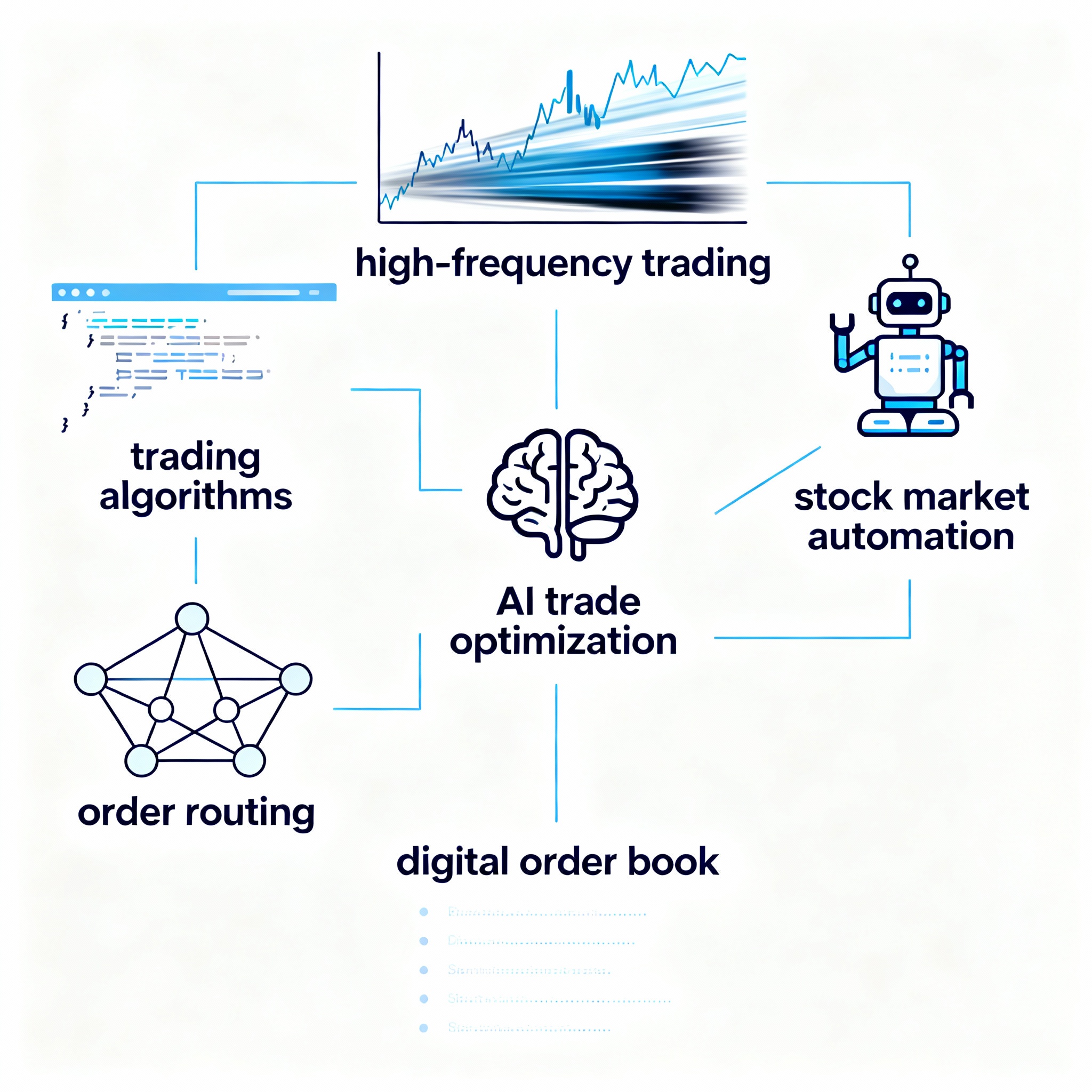
    Trading algorithms have revolutionized financial markets, transforming the landscape from human-dominated trading floors to lightning-fast electronic execution environments where billions of orders are processed in microseconds. These sophisticated computer programs analyze market data, identify trading opportunities, and execute orders with minimal human intervention, operating at speeds impossible for manual traders. High-frequency trading (HFT) firms deploy cutting-edge algorithms that capitalize on minute price discrepancies, while AI-driven systems continuously learn from market patterns to optimize order routing and minimize trading costs. Understanding modern algorithmic trading—from the mechanics of HFT strategies to AI-powered order execution—is essential for anyone seeking to comprehend how contemporary financial markets actually operate.

    The Mechanics of Algorithmic Trading

    Algorithmic trading refers to the use of computer programs to execute trading strategies automatically based on predefined rules and market conditions. At its core, a trading algorithm continuously monitors market data feeds—price quotes, order book depth, trade volumes, news feeds—and applies mathematical models to identify trading opportunities. When conditions match the algorithm’s criteria, it automatically generates and submits orders to exchanges, often splitting large orders into smaller pieces to minimize market impact. The sophistication ranges from simple rule-based systems (“buy when the 50-day moving average crosses above the 200-day”) to complex machine learning models that adapt to changing market regimes in real-time.

    High-Frequency Trading Strategies

    High-frequency trading represents the most technologically advanced subset of algorithmic trading, characterized by extremely high speeds, short holding periods (often measured in seconds or milliseconds), and massive order volumes. HFT firms invest heavily in ultra-low-latency infrastructure—co-locating servers next to exchange data centers, using specialized network hardware, and optimizing code to the nanosecond level. The goal is to be faster than competitors, gaining first access to market information and trading opportunities.

    Key HFT strategies include:

    Market Making: HFT firms continuously post bid and ask quotes, profiting from the bid-ask spread while providing liquidity. Their algorithms dynamically adjust quotes based on inventory positions and market volatility.

    Latency Arbitrage: Exploiting speed advantages to trade on price information before slower participants can react. For example, if a price change occurs on one exchange, HFT algorithms can trade on other exchanges before those prices adjust.

    Statistical Arbitrage: Identifying short-term pricing inefficiencies between correlated instruments and executing simultaneous buy/sell orders to capture the spread.

    Liquidity Detection: Using algorithms to detect large hidden orders in dark pools or fragmented across venues, then trading ahead of anticipated price movements.

    AI-Driven Order Routing and Execution

    Modern trading isn’t just about speed—it’s about intelligence. AI-driven order routing systems use machine learning to determine the optimal way to execute large orders while minimizing market impact and transaction costs. These systems analyze historical execution data, current market conditions, and real-time liquidity across multiple venues to make split-second routing decisions.

    Key AI optimization techniques include:

    Venue Selection: Algorithms learn which trading venues offer the best execution quality for different order types and market conditions, dynamically routing orders to exchanges, dark pools, or alternative trading systems.

    Order Slicing: AI models determine optimal order size and timing to minimize market impact, breaking large orders into smaller child orders executed over time.

    Price Prediction: Machine learning models forecast short-term price movements to optimize entry and exit timing, improving execution prices.

    Reinforcement Learning: Advanced algorithms learn from past execution outcomes, continuously improving their strategies through trial and error in simulated and live environments.

    Key Formulas and Metrics

    Implementation Shortfall:

    Implementation Shortfall = (Execution Price – Decision Price) × Shares Traded

    This measures the cost of execution delay and market impact, representing the difference between the ideal execution price and the actual achieved price.

    Volume-Weighted Average Price (VWAP):

    VWAP = Σ(Price × Volume) / Σ(Volume)

    Algorithms often aim to execute orders at prices better than the VWAP benchmark, which represents the average price weighted by trading volume over a specific time period.

    Sharpe Ratio for Algorithmic Strategies:

    Sharpe Ratio = (Rstrategy – Rrf) / σstrategy

    Where Rstrategy is the strategy return, Rrf is the risk-free rate, and σstrategy is the standard deviation of strategy returns. Higher Sharpe ratios indicate better risk-adjusted performance.

    Real-World Examples: Citadel and Renaissance Technologies

    Citadel Securities operates one of the world’s most sophisticated algorithmic trading operations, executing approximately 47% of all U.S. retail equity volume. The firm’s technology infrastructure processes millions of quotes per second, using machine learning algorithms to optimize execution across fragmented markets. Citadel’s algorithms dynamically adjust to market conditions, providing liquidity while managing inventory risk through sophisticated hedging strategies. Their order routing intelligence determines optimal execution venues in real-time, minimizing costs for retail order flow they handle.

    Renaissance Technologies, founded by mathematician James Simons, pioneered quantitative algorithmic trading with their flagship Medallion Fund, which has delivered extraordinary returns (averaging 66% annual returns before fees from 1988-2018). Renaissance employs hundreds of PhDs in mathematics, physics, and computer science who develop proprietary algorithms based on statistical patterns discovered through massive data analysis. Their models identify subtle correlations and market inefficiencies invisible to human traders, executing thousands of automated trades daily across global markets. The firm’s success demonstrates the power of combining advanced mathematics, big data analytics, and algorithmic execution.

    Dark Pools and Order Flow Internalization

    Dark pools are private trading venues where large institutional orders can be executed away from public exchanges, preventing information leakage that could move prices against the trader. Algorithmic trading systems routinely access dark pools as part of smart order routing strategies, seeking hidden liquidity that won’t impact public market prices. However, the opacity of dark pools has raised concerns about fairness—sophisticated algorithms can detect patterns in dark pool activity and potentially trade ahead of large orders.

    Order flow internalization occurs when broker-dealers execute client orders against their own inventory or match them with other client orders rather than sending them to public exchanges. Algorithmic systems manage this process, determining when internalization provides better execution than external routing. Critics argue this creates conflicts of interest, while proponents claim it often results in price improvement for retail investors.

    Regulatory Considerations and Market Impact

    The rise of algorithmic and high-frequency trading has prompted regulatory scrutiny. The 2010 Flash Crash—when the Dow Jones Industrial Average plunged nearly 1,000 points in minutes before rapidly recovering—highlighted risks of algorithmic trading gone awry. Regulators have implemented circuit breakers, minimum quote durations, and enhanced monitoring to detect manipulative algorithmic strategies like spoofing (placing fake orders to manipulate prices) and layering.

    The SEC’s Regulation NMS governs order routing and best execution requirements, while MiFID II in Europe mandates algorithm testing and kill switches. Exchanges implement co-location policies and maker-taker fee structures that influence algorithmic behavior. Understanding this regulatory framework is crucial for developing compliant trading algorithms.

    Glossary

    Trading Algorithm: A computer program that automatically executes trading strategies based on predefined rules, market data, and mathematical models, minimizing human intervention in the trading process.

    High-Frequency Trading (HFT): A type of algorithmic trading characterized by extremely high speeds, short holding periods, and large order volumes, typically seeking to profit from small price discrepancies across markets.

    Order Routing: The process of determining which trading venue (exchange, dark pool, or alternative system) will provide the best execution for a particular order, often optimized using AI and machine learning.

    Latency Arbitrage: A trading strategy that exploits speed advantages to profit from temporary price discrepancies between markets before slower participants can react to new information.

    Dark Pool: A private trading venue where institutional investors can execute large orders anonymously, away from public exchanges, to minimize market impact and information leakage.

    Test Algorithmic Strategies in Our Sandbox!

    Ready to experience algorithmic trading firsthand? Try our interactive trading sandbox where you can test algorithmic strategies, experiment with order routing logic, and see how different execution algorithms perform under various market conditions. Understanding algorithmic trading mechanics empowers you to make more informed investment decisions and better comprehend the technology driving modern financial markets.

  • Understanding Market Makers: Liquidity, Bid-Ask Spreads, and Price Stabilization

    Understanding Market Makers: Liquidity, Bid-Ask Spreads, and Price Stabilization

    The Essential Role of Liquidity Providers in Financial Markets

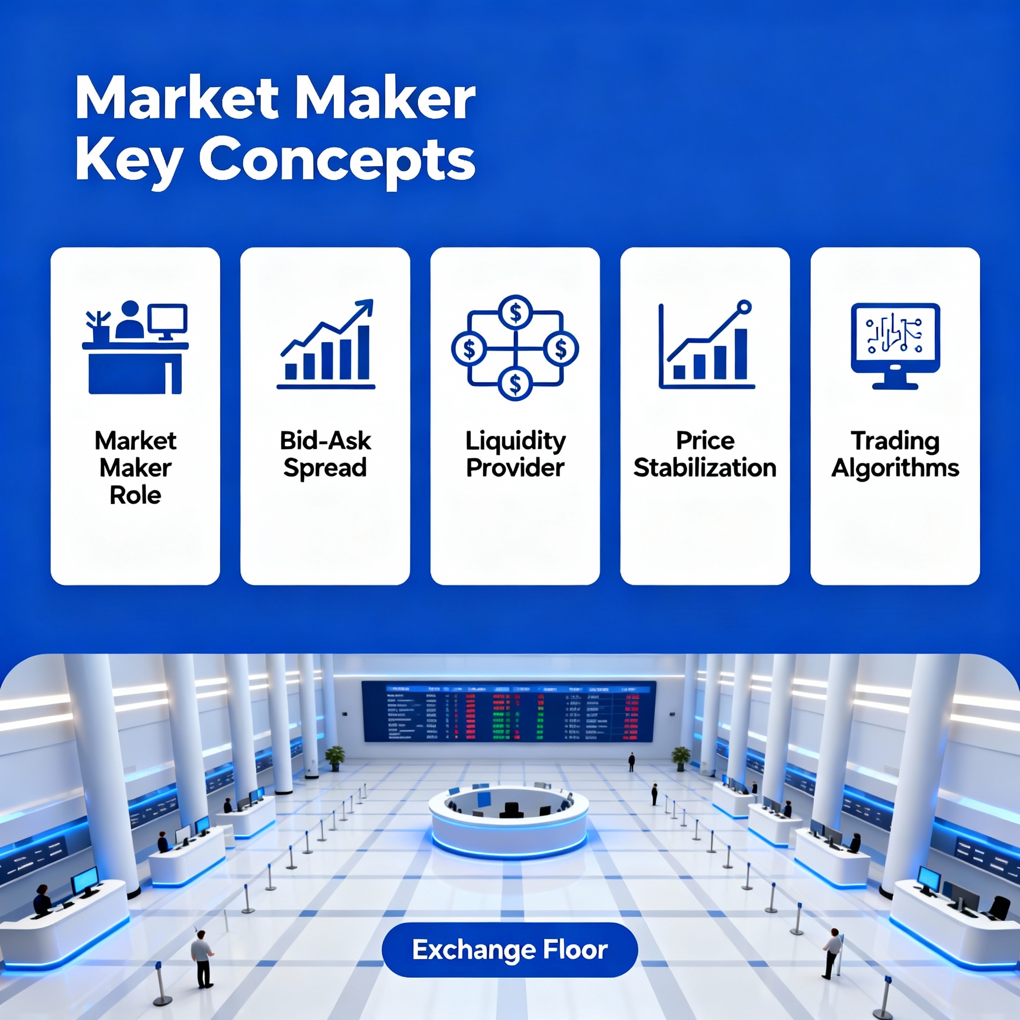
    Market makers are specialized financial firms or individuals that stand ready to buy and sell securities at publicly quoted prices, ensuring that markets remain liquid and functional even during periods of low trading activity. Acting as intermediaries between buyers and sellers, market makers provide continuous two-sided quotes—both bid prices (where they’ll buy) and ask prices (where they’ll sell)—creating immediate execution opportunities for traders. By absorbing temporary supply-demand imbalances and maintaining orderly price discovery, market makers reduce volatility, narrow bid-ask spreads, and enable efficient capital allocation across financial markets. Understanding how market makers operate, manage risk, and profit from their activities is essential for anyone seeking to comprehend modern market microstructure.

    The Mechanics of Market Making

    Market making operates on a deceptively simple principle: buy low, sell high, and do it repeatedly throughout the trading day. Market makers continuously post bid and ask quotes for securities they’re assigned to cover, creating a standing offer to transact. When an investor wants to buy shares immediately, they purchase at the market maker’s ask price; when selling, they receive the market maker’s bid price. The difference between these two prices—the bid-ask spread—represents the market maker’s gross profit per transaction before costs.

    Understanding the Bid-Ask Spread

    The bid-ask spread serves multiple functions in market structure. It compensates market makers for the immediacy service they provide, covering operational costs (technology, compliance, personnel) and adverse selection risk—the probability that they’re trading with someone who has superior information. Spreads vary significantly across securities based on factors like trading volume, volatility, and information asymmetry.

    Bid-Ask Spread Formula:

    Spread = Ask Price – Bid Price

    Percentage Spread = ((Ask – Bid) / Midpoint) × 100

    For example, if a stock has a bid of $50.00 and an ask of $50.10, the absolute spread is $0.10 and the percentage spread is 0.20%. High-volume, liquid stocks like Apple might have spreads of just $0.01 (0.002%), while thinly traded small-cap stocks might see spreads of 5% or more.

    Inventory Management and Risk Control

    Market makers face continuous inventory risk. When they buy shares at the bid, they hope to quickly sell at the ask, but if market prices decline before they can offload their position, they incur losses. Conversely, if they sell short at the ask and prices rise before they can buy back, they also lose money. Effective inventory management is therefore critical to market maker profitability.

    Market makers employ sophisticated hedging strategies and algorithmic systems to manage inventory risk. They might hedge directional exposure using index futures or options, dynamically adjust their bid-ask spreads based on current inventory positions (widening spreads when they hold large positions to discourage further accumulation), or trade with other market makers to rebalance positions.

    Inventory Risk Premium:

    Required Spread ≥ (σ√(T/2)) + Transaction Costs

    Where σ is volatility and T is expected holding period. Higher volatility or longer expected holding periods demand wider spreads to compensate for increased inventory risk.

    Trading Algorithms and Price Stabilization

    Modern market making relies heavily on trading algorithms that continuously monitor order books, news feeds, and market conditions to update quotes milliseconds after new information arrives. These algorithms employ statistical models and machine learning to predict short-term price movements and optimize quote placement. The most sophisticated market makers operate across multiple venues simultaneously, providing liquidity on lit exchanges, dark pools, and alternative trading systems while managing consolidated risk across all platforms.

    Market makers contribute significantly to price stabilization by absorbing temporary imbalances between buy and sell orders. When excessive selling pressure emerges, market makers step in as buyers (though at lower bid prices); when buying pressure dominates, they become sellers (at higher ask prices). This countercyclical behavior dampens price volatility and reduces the magnitude of price swings that would occur in their absence. However, during extreme market stress—such as the 2010 Flash Crash or March 2020 COVID panic—even market makers can withdraw liquidity when their risk management systems trigger circuit breakers, potentially exacerbating volatility.

    Real-World Examples and Market Participants

    Major market makers include firms like Citadel Securities, Virtu Financial, Jane Street, and Two Sigma Securities, which together handle significant percentages of daily U.S. equity trading volume. On the NASDAQ, designated market makers have explicit obligations to maintain continuous quotes within specified spreads. On the NYSE, Designated Market Makers (DMMs) combine electronic market making with human judgment, particularly during market opens, closes, and periods of significant imbalance.

    Consider Citadel Securities, which reports executing approximately 47% of all U.S.-listed retail volume across more than 8,900 securities. The firm’s technology infrastructure can handle millions of quotes per second, adjusting prices based on microsecond changes in market conditions. In foreign exchange markets, banks like J.P. Morgan and Citigroup act as market makers, posting continuous bid-ask spreads for currency pairs and profiting from the cumulative spread across billions of dollars in daily trading volume.

    Broker-Dealer Distinction and Regulatory Framework

    Market makers typically operate as broker-dealers, registered with the SEC and FINRA, subject to capital requirements, trade reporting obligations, and best execution standards. The distinction between broker (agent executing customer orders) and dealer (principal trading from own account) is important: as dealers, market makers bear inventory risk and price risk that brokers do not. Regulations like Reg NMS (National Market System) govern quote display requirements, trade-through prohibitions, and access to displayed quotations, creating the framework within which market makers operate.

    Glossary

    Market Maker: A firm or individual that continuously quotes both buy (bid) and sell (ask) prices for financial instruments, standing ready to trade at those prices and thereby providing liquidity to the market.

    Bid-Ask Spread: The difference between the highest price a buyer is willing to pay (bid) and the lowest price a seller is willing to accept (ask) for a security, representing the market maker’s gross profit per transaction.

    Liquidity: The degree to which an asset can be quickly bought or sold in the market at stable prices. High liquidity means transactions can occur rapidly with minimal price impact.

    Price Stabilization: The process by which market makers and other participants dampen excessive price volatility by providing countercyclical liquidity—buying during selling pressure and selling during buying pressure.

    Broker-Dealer: A financial entity that acts both as a broker (executing trades on behalf of clients) and dealer (trading securities from its own account), subject to SEC and FINRA regulation.

    Try Market Making in Our Stock Trading Sandbox!

    Ready to experience market making firsthand? Try our interactive stock trading sandbox where you can simulate posting bid-ask quotes, managing inventory risk, and learning how liquidity providers operate in real market conditions. Understanding market microstructure empowers you to make more informed trading decisions and better comprehend the dynamics behind every trade you execute.

  • Essential Stock Market Indices and Benchmarks: S&P 500, Dow Jones, Global Comparisons

    Essential Stock Market Indices and Benchmarks: S&P 500, Dow Jones, Global Comparisons

    Understanding the Benchmarks That Define Market Performance

    Stock market indices serve as essential barometers of financial market health, providing investors with standardized benchmarks to measure performance, compare investments, and understand broad market trends. From the iconic S&P 500 and Dow Jones Industrial Average in the United States to global indices like the FTSE 100 and Nikkei 225, these carefully constructed baskets of securities offer invaluable insights into economic conditions and investor sentiment. Understanding how indices are calculated, rebalanced, and utilized is fundamental to making informed investment decisions and contextualizing individual stock or portfolio performance against the broader market.

    The Mechanics of Stock Market Indices

    At their core, stock market indices aggregate the prices of multiple stocks into a single metric that represents the performance of a specific market segment or the entire market. The methodology behind index construction varies significantly. Price-weighted indices like the Dow Jones Industrial Average give greater weight to stocks with higher share prices, while market-cap-weighted indices such as the S&P 500 allocate weight based on each company’s total market capitalization. Equal-weighted indices, by contrast, give each constituent stock the same influence regardless of its price or size. These methodological differences profoundly impact index behavior and the types of investment strategies they support.

    Calculation Methods Explained

    Price-Weighted Index Formula:

    Index Value = (Sum of Stock Prices) / Divisor

    The Dow Jones Industrial Average uses this method, where a stock trading at $200 has twice the impact of a stock trading at $100, regardless of company size.

    Market-Cap-Weighted Index Formula:

    Index Value = (Sum of (Stock Price × Shares Outstanding)) / Base Market Cap × Base Index Value

    The S&P 500 employs this methodology, meaning Apple or Microsoft with trillion-dollar market caps significantly influence the index more than smaller companies.

    Rebalancing and Index Maintenance

    Index rebalancing is the periodic adjustment of index constituents to maintain the index’s representativeness and adherence to its stated methodology. For market-cap-weighted indices, rebalancing ensures that stock weights accurately reflect current market valuations. The S&P 500 Index Committee reviews constituents quarterly, adding companies that meet specific criteria (such as market cap thresholds, liquidity requirements, and financial viability) while removing those that no longer qualify. Rebalancing events can trigger significant trading volume as index funds and ETFs must buy or sell stocks to match the new composition, creating price pressure and liquidity demands that sophisticated investors closely monitor.

    Sector Impact and Representation

    Modern indices typically organize constituents into sectors (Technology, Healthcare, Financials, Energy, etc.), and sector weightings significantly influence index performance. In recent years, the Technology sector’s explosive growth has dramatically increased its representation in major U.S. indices. As of late 2024, Technology companies constitute approximately 30% of the S&P 500’s market cap, meaning tech stock movements disproportionately affect overall index performance. This sector concentration introduces sector-specific risks; a downturn in Technology can drag down the entire index despite strength in other sectors. Investors must understand sector dynamics when using indices as benchmarks or investment vehicles.

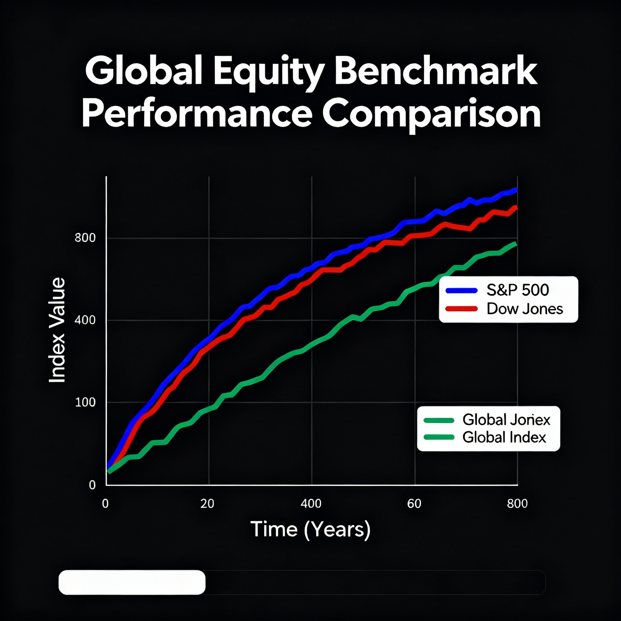
    Global Equity Benchmarks: A Comparative Overview

    While U.S. indices dominate global financial discourse, international benchmarks provide critical insights into global markets:

    • FTSE 100 (UK): Tracks the 100 largest companies listed on the London Stock Exchange, heavily weighted toward Financial Services, Energy, and Consumer Goods sectors.
    • DAX (Germany): A performance index of 40 major German blue chip companies, representing Europe’s largest economy.
    • Nikkei 225 (Japan): A price-weighted index of 225 top-rated companies on the Tokyo Stock Exchange, providing a window into Asia’s second-largest economy.
    • Hang Seng Index (Hong Kong): Represents the largest companies on the Hong Kong Stock Exchange, with significant exposure to Chinese financial and technology firms.
    • MSCI Emerging Markets Index: A market-cap-weighted index capturing large and mid-cap representation across 24 emerging market countries.

    Historical Performance and Lessons

    Examining historical index performance reveals important investment principles. The S&P 500 has delivered an average annual return of approximately 10% since its inception in 1957, though individual years vary dramatically. The 2008 financial crisis saw the S&P 500 decline 37%, while 2013 brought a 32% gain. These fluctuations underscore the importance of long-term perspective and diversification. Global comparisons show that U.S. indices have significantly outperformed most international benchmarks over the past decade, driven by technology sector dominance and robust corporate earnings growth. However, past performance never guarantees future results, and geopolitical shifts, regulatory changes, or economic cycles can rapidly alter relative performance among global indices.

    Key Takeaways for Investors

    • Index methodology (price-weighted vs. market-cap-weighted vs. equal-weighted) fundamentally affects index behavior and investment outcomes.
    • Rebalancing events create trading opportunities and risks as index funds adjust their holdings.
    • Sector concentration, particularly in Technology, has increased the correlation between individual mega-cap stocks and overall index performance.
    • Global indices provide diversification benefits and exposure to different economic cycles, regulatory environments, and currency movements.
    • Historical performance data should inform but not dictate investment decisions; understanding the underlying economic and corporate fundamentals matters more than chasing past returns.

    Glossary

    S&P 500: A market-capitalization-weighted index of 500 leading publicly traded companies in the United States, widely regarded as the best single gauge of large-cap U.S. equities.

    Benchmark: A standard against which the performance of an investment portfolio, security, or investment manager can be measured. Common benchmarks include stock market indices like the S&P 500 or Dow Jones Industrial Average.

    Rebalancing: The process of realigning the weightings of a portfolio or index by periodically buying or selling assets to maintain the desired asset allocation or index methodology.

    Blue Chip: Stock of a well-established, financially sound company with a history of reliable performance, typically included in major stock indices. Examples include companies in the Dow Jones Industrial Average.

    Index Fund: A type of mutual fund or exchange-traded fund (ETF) designed to track the performance of a specific index by holding the same securities in the same proportions as the index.

    Compare Indices and Analyze Trends

    Ready to put your knowledge into practice? Compare indices in our interactive sandbox or analyze historical trends across global equity benchmarks. Understanding these fundamental tools empowers you to make more informed investment decisions and better contextualize market movements within the broader financial landscape.

  • Follow-On Offerings (FPOs): Raising Additional Equity After the IPO

    Follow-On Offerings (FPOs): Raising Additional Equity After the IPO

    Executive Summary

    • What it is: A follow-on offering (FPO) issues additional shares after the IPO.
    • Why it matters: Funds growth, M&A, or deleveraging while increasing float and liquidity.
    • Types: Primary (new shares, dilutive) vs. Secondary (existing holders sell, non-dilutive).

    Core Structure
    1) Use of Proceeds

    • Primary FPOs raise capital for expansion, R&D, capex, acquisitions, or balance sheet repair.
    • Secondary offerings provide liquidity for insiders/VCs without raising new company cash.

    2) Deal Formats

    • Fully marketed: 2–4 day investor education; wider distribution; potential pricing support.
    • Accelerated bookbuild (ABB): Overnight/one-day wall-cross; speed reduces market risk.
    • Bought deal: Underwriter purchases all shares, assuming market risk for a fee.

    3) Pricing Mechanics

    • Discount to last close/ VWAP to incentive uptake; typical 2–8% depending on size/volatility.
    • Key determinants: Offer size as % of float, recent performance, investor mix, lock-up context.
    • Allocation: Tiered between long-only, hedge funds, and existing holders to stabilize post-trade.

    4) Dilution and Float

    • Primary FPO increases share count; EPS dilution unless proceeds create value above cost of capital.
    • Larger public float can tighten spreads, deepen book, and improve index eligibility.

    5) Regulatory & Documentation

    • Shelf registration (e.g., SEC Form S-3) enables rapid takedowns.
    • Prospectus supplements detail use of proceeds, risk factors, and underwriting terms.

    6) Execution Timeline

    • Pre-soundings and wall-cross → launch → bookbuild → price → allocate → T+1 settlement.
    • Stabilization: Greenshoe/over-allotment supports aftermarket performance.

    Worked Example
    Company XYZ runs an ABB for 15M shares (~7% float) at 4% discount to last close.

    • Proceeds: $450M to repay revolver and fund AI capex.
    • Impact: EPS -2% near-term; leverage drops from 2.4x to 1.6x; liquidity improves.

    Investor Checklist

    • Evaluate dilution vs. ROIC on proceeds deployment.
    • Scrutinize discount vs. historical norms and deal size.
    • Assess lock-ups, insider participation, and underwriter quality.
    • Model pro forma ownership, leverage, and EPS.

    Glossary

    • ABB: Rapid bookbuild to price overnight/next-day.
    • Greenshoe: Option to sell 15% extra shares for stabilization.
    • Shelf: Registration enabling quick securities issuance.

    SEO Keywords
    follow-on offering, FPO, secondary offering, accelerated bookbuild, greenshoe, shelf registration, dilution, float, pricing discount, use of proceeds

    CTA
    Want pro-grade ECM insights weekly? Subscribe for term sheets, case studies, and playbooks.

  • The Secondary Market Explained: Where Stocks Trade After the IPO

    The Secondary Market Explained: Where Stocks Trade After the IPO

    Executive Summary

    • What it is: The secondary market is where existing securities trade among investors after the initial public offering (IPO).
    • Why it matters: It provides liquidity, price discovery, and efficient capital allocation across the economy.
    • Who uses it: Retail investors, institutions, market makers, high-frequency traders, and corporate insiders post lock-up.

    Core Concepts
    1) Primary vs. Secondary Market

    • Primary: Company issues new shares to raise capital (e.g., IPO, follow-on offering).
    • Secondary: Shares trade between investors on exchanges (NYSE, Nasdaq) or OTC venues; company doesn’t directly receive proceeds.

    2) Venues and Microstructure

    • Lit exchanges: Central limit order books (CLOBs) match bids/offers transparently.
    • Dark pools: Alternative trading systems offering midpoint/hidden liquidity for size.
    • OTC/Market maker platforms: Quote-driven with dealer intermediation.
    • Auction opens/closes: Opening and closing auctions concentrate liquidity and set reference prices.

    3) Order Types and Execution

    • Market order: Fill immediately at best available price; priority is speed over price.
    • Limit order: Execute at your stated price or better; priority is price control over immediacy.
    • Stop/Stop-limit: Triggered after a stop price; used for risk control.
    • Time-in-force: Day, IOC, FOK, GTC determine order lifespan.
    • Smart order routing: Brokers split orders across venues for best execution.

    4) Liquidity and Spreads

    • Liquidity depth reduces impact cost; measured by quoted/realized spreads and book depth.
    • Bid-ask spread narrows with competition, volume, and tighter tick sizes.
    • Market makers supply two-sided quotes; earn spread and rebates, manage inventory/risk.

    5) Price Discovery and Market Quality

    • Continuous trading plus auction mechanisms aggregate information into prices.
    • Market quality metrics: Volatility, spreads, depth, price efficiency, and throughput.
    • Events affecting prices: Earnings, macro data, sector news, rebalances, insider flows.

    6) Settlement Cycle (T+1)

    • US equities settle T+1: trade date plus one business day.
    • Operations: Trade capture, clearing via NSCC, custody updates at DTC, cash/securities delivery.
    • Fails management: Buy-ins and penalties discourage settlement failures.

    7) Short Selling and Securities Lending

    • Locate/borrow shares via lending markets (agents, beneficial owners).
    • Collateralized borrow, daily mark-to-market; borrow cost varies by scarcity.
    • Uptick/SSR rules can restrict shorts in extreme down moves.

    8) Risk and Controls

    • Slippage and market impact from order size/urgency.
    • Hidden costs: Spreads, fees, and information leakage.
    • Guardrails: Circuit breakers, LULD bands, kill-switches, margin rules.

    Worked Example
    Scenario: Investor wants to buy 10,000 shares of ABC at $50.

    • Approach A (market order): Immediate fill, average $50.05; higher impact cost.
    • Approach B (limit $50): Partial fills over day; average $49.98; execution risk remains.
    • Router blend: Slices to exchanges/dark pools, pegs at midpoint; minimizes footprint.

    Checklist for Practitioners

    • Define objective: immediacy vs. price control.
    • Choose order type/time-in-force accordingly.
    • Monitor venue fills, routing logic, and slippage.
    • Use auction liquidity at open/close for larger trades.

    Glossary

    • CLOB: Centralized book of bids/offers ranked by price-time priority.
    • LULD: Limit Up/Limit Down volatility guardrails.
    • NSCC/DTC: US clearing/depository infrastructure for equity settlement.
    • Midpoint peg: Order priced at midpoint of NBBO.

    SEO Keywords
    secondary market, post-IPO trading, stock exchanges, dark pools, market makers, bid-ask spread, T+1 settlement, short selling, liquidity, order types, price discovery

    Meta Description (120–155 chars)
    Understand how the secondary market works post‑IPO: venues, order types, liquidity, price discovery, and T+1 settlement.

    CTA
    Ready to master execution strategy? Subscribe for weekly market microstructure and trading insights.

  • How IPOs Shape the Equity Capital Market: From Private to Public Powerhouses

    How IPOs Shape the Equity Capital Market: From Private to Public Powerhouses

    Transform Your Company Through Public Listing: Unlocking Capital, Credibility, and Growth

    An Initial Public Offering (IPO) represents one of the most transformative moments in a company’s lifecycle. When a private company decides to go public, it doesn’t just sell shares—it fundamentally reshapes its position within the equity capital market, unlocks new growth trajectories, and creates ripple effects throughout the financial ecosystem.

    Introduction: The Gateway to Capital Markets

    The equity capital market serves as the vital infrastructure connecting companies seeking capital with investors seeking returns. At the heart of this ecosystem lies the IPO process—the mechanism through which privately-held companies transition to publicly-traded entities. This transformation enables companies to raise substantial capital from institutional and retail investors while providing liquidity to early investors and employees.

    Understanding IPOs is essential for anyone serious about equity markets. Whether you’re an aspiring investor, a finance professional, or an entrepreneur considering taking your company public, grasping how IPOs function reveals the fundamental architecture of modern capital markets.

    Core Insights: The IPO Mechanics

    The IPO Process: Companies typically work with investment banks (underwriters) who help determine the offering price, manage regulatory compliance, and distribute shares to investors. The process involves extensive due diligence, SEC registration (Form S-1 in the U.S.), roadshows to attract institutional investors, and finally, the pricing and listing on a stock exchange.

    Pricing Mechanisms: Investment banks use various valuation methods including comparable company analysis, discounted cash flow models, and precedent transactions. The final IPO price balances maximizing capital raised with ensuring strong first-day trading performance to satisfy both the company and new investors.

    Market Impact: IPOs inject liquidity into the equity capital market, create new investment opportunities, and often signal broader market sentiment. Large IPOs can influence sector valuations and investor appetite for similar companies.

    Educational Layer: Key Takeaways

    1. Underpricing Phenomenon: Research shows that IPOs are typically underpriced by 10-15% on average, meaning first-day returns often exceed the offering price. This intentional underpricing leaves “money on the table” for investors as an incentive and ensures successful market debut.

    2. The Lock-Up Period: Insiders and early investors typically face a 90-180 day lock-up period preventing them from selling shares. This restriction protects against sudden supply shocks but can create price volatility when lock-ups expire.

    3. Valuation Formula – Price-to-Earnings Approach:
    IPO Valuation = Projected Annual Earnings × Industry Average P/E Ratio
    Example: If a company projects $50M in earnings and the industry P/E is 20x, the estimated valuation would be $1 billion.

    Real-World Example: Major IPOs That Shaped Markets

    Saudi Aramco (2019): The world’s largest IPO raised $25.6 billion, valuing the company at $1.7 trillion. This offering demonstrated how national champions can leverage public markets while maintaining strategic government control.

    Alibaba (2014): Raised $25 billion on the NYSE, becoming the largest U.S. IPO. The offering provided Western investors access to China’s e-commerce boom and established a template for Chinese tech companies accessing global capital.

    Snowflake (2020): Debuted at $120 per share (versus $120 IPO price that was already raised from $100-110 range), jumping to $245 on day one. This 111% pop illustrated extreme investor demand for cloud data companies and the potential underpricing that benefits initial buyers.

    AI Insight: Predictive IPO Analysis

    Advanced AI models now analyze IPO performance predictors by examining factors including:

    • Venture capital backing quality and reputation
    • Market sentiment and volatility indices (VIX) at offering time
    • Company fundamentals: revenue growth, profitability trajectory, competitive moat
    • Underwriter prestige and allocation strategies
    • Industry tailwinds and comparable company performance

    Machine learning algorithms can identify patterns suggesting whether an IPO will outperform or underperform in the first year, though market unpredictability ensures no model achieves perfect accuracy.

    Key Terms / Glossary

    IPO (Initial Public Offering): The first sale of stock by a private company to the public, transitioning the company to publicly-traded status.

    Underwriter: Investment bank that manages the IPO process, assumes risk by purchasing shares from the company, and resells them to investors.

    Prospectus: Legal document (SEC Form S-1) detailing company financials, business model, risks, and offering terms; required for all public offerings.

    Book Building: Process where underwriters gauge investor demand at various price points to determine the final IPO price.

    Greenshoe Option: Over-allotment provision allowing underwriters to sell up to 15% additional shares if demand exceeds expectations, stabilizing the stock price.

    Call to Action

    Ready to deepen your understanding of equity markets? Explore our IPO simulation sandbox where you can practice evaluating offerings, setting price targets, and building allocation strategies without risking real capital.

    Read next: “The Psychology of Market Timing: Why Most Investors Buy High and Sell Low” to understand behavioral factors that influence IPO investment decisions.

    Stay ahead of the market. Subscribe to our newsletter for weekly insights on equity capital markets, IPO analysis, and investment strategies.